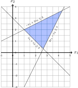
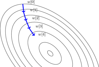
Quadratic Programming

Quadratic Programming is a combination of multiple mathematical concepts. Quadratic approximation (Taylor Series), Constrained function as well cost/loss optimization. Combined, it creates a convex optimization problem. Meaning that the problem can only be solved if and only if the problem can be represented as a convex problem. Additionally, the solution will only be within the convex region of the problem.

Quadratic Programming is formulated as the following:

$\min_{x} \frac{1}{2}x^TQx + C^Tx$

$\textrm{s.t} \quad Ax \le b$

The formula states that, find $x$ that will yield the smallest number, and minimize $x$ , while satisfying the constrained linear equation $Ax \le b$ . Where $s.t$ stands for subjected to.

When unfolding the linear algebraic expression we get the following:

$\min_{x} a_0x^2_0+a_1x^2_1+...+a_nx^2_n+b_0x_0+b_1x_1+...+b_nx_n+c$

The function with the min is the loss function that states how good the $x$ value is. It is used as for expressing what the optimization should attempt to optimize as well if going in the right direction.

Finally, the $\frac{1}{2}x^TQx + C^Tx$ is the quadratic approximation function that describes the optimization itself. Quadratic Programming is just a special case of using Quadratic Approximation and can be expressed as Polynomial Programming for generalizing.

Linear Programming

It should be notated that a subset of the quadratic programming cost optimization function is from linear programming. Thus it is suggested to learn it before quadratic programming.

$\min_{x} b_0x_0+b_1x_1+...+b_nx_n+c$

$\textrm{s.t} \quad Ax \le d$

Taylor Series – Approximation

The Quadratic approximation is derived from the Taylor Series, which is a definition of how a function can be re-expressed as the sum of an infinite sequence of derivative functions at a particular point. See the following definition:

$f(x)=\sum^{\infty}_{n=0}\dfrac{f^{(n)}(a)}{n!}(x-a)^n$

For instance, a sine function, $f(x) = sin(x)$ , can be expressed as an infinite polynomial expression.
However, it should be noted that working with infinite sequences is very much restricted when solving purely as a mathematical problem. Whereas applied mathematics in the real-world problem may not be able to make use of infinite sequence since it would require infinite function.
Instead, since this is done in the real world and an infinite sequence is impossible, instead an approximate version can be opted for and computed. Where the amount of error will be proportional to what degree of the Taylor Series is used as well as the distance from the sampled point and the point that the approximate function is based on.

See the following Taylor Series definition:

$f(x)\thickapprox\sum^{K}_{n=0}\dfrac{f^{(n)}(a)}{n!}(x-a)^n$

Linear Approximation

For a linear approximation, it will essentially become the tangent line. Since it will have the shape of a linear function. Additionally, it can for any given dimension, which effectively makes it a hyperplane. Though a linear approximation is limited by that it is only good for the problems that have a linear relationship.

$f(x) = ax +c$

Taylor Series

The Linear Approximation is derived from the Taylor Series, see the following.

$f(x) = \sum^{K=2}_{n=0}\dfrac{f^{(n)}(a)}{n!}(x-a)^n$

$f(x) = c + ax = \frac{f^{(0)}(a)}{0!}(x - a)^0 + \frac{f^{(1)}(a)}{1!}(x - a)^1$

The Taylor can be reduced into a condensed Algebraic equation, that is the same shape as the linear equation:

$L_f(x) = f(x_0) + \triangledown f(x_0)\cdot(x -x_0)$

Quadratic Approximation

The Quadratic approximation is the next level from the linear approximation one. It approximates the function around a certain point with a higher-level approximation.
It has the shape of a quadratic equation, see the following:

$f(x) = ax^2 + bx + c$

Deriving the Quadratic Approximation from the Taylor series gives the following.

$f(x) = \sum^{K=3}_{n=0}\dfrac{f^{(n)}(a)}{n!}(x-a)^n$

$f(x) = c + bx + ax^2 + = \frac{f^{(0)}(a)}{0!}(x - a)^0 + \frac{f^{(1)}(a)}{1!}(x - a)^1 + \frac{f^{(2)}(a)}{2!}(x - a)^2$

The Quadratic approximation in linear-algebraic form can be expressed as follows:

$Q_f(x) = f(x_0) + \triangledown f(x_0)\cdot(x -x_0) + \frac{1}{2}(x-x_0)^TH_f(x_0)(x - x_0)$

The expression $\triangledown f(x_0)$ First order Partial derivative in respect for all the variables of $x$ . It will have the shape of a vector.
The expression $H_f(x_0)$ is the Hessian Matrix, which contains all possible combinations of partial derivatives as a square matrix.

Partial Derivative

Partial Differential is rather straightforward to calculate. The first-order ordinary derivative is calculated for each of the variables individually. Resulting in a vector/list of derivatives equal to the number of variables.
For instance, given the following function with two variables.

$f(x,y) = x^2y + y^2x$

Thus computing the individual variable’s derivatives gives the following set of functions:

$\frac{\partial f}{\partial x} = 2xy + y^2$

$\frac{\partial f}{\partial y} = x^2 + 2yx$

Finally, it can be generalized as the following:

$\begin{bmatrix}\frac{\partial f}{\partial v_0}\\\frac{\partial f}{\partial v_1}\\\frac{\partial f}{\partial v_2}\\\cdots\\\frac{\partial f}{\partial v_{n-1}}\\\end{bmatrix} \le (\frac{\partial f}{\partial v_0},\frac{\partial f}{\partial v_1},\frac{\partial f}{\partial v_2},\cdots\frac{\partial f}{\partial v_{n-1}} )$

Hessian Matrix

Hessian Matrix is the second-order ordinary partial differential, expressed as a matrix that contains all the combinations of second-order partial differential. See the following for a two variables example function as a Hessian Matrix:

$\begin{bmatrix}\frac{\partial^2 f}{\partial x^2} & \frac{\partial^2 f}{\partial x \partial y}\\\frac{\partial^2 f}{\partial x \partial y} & \frac{\partial^2 f}{\partial y^2}\end{bmatrix}$

Since Hessian Matrix is a square matrix, when multiplied by the vector, it produces a vector.

Constraint

Constraints are additional conditions that a mathematical problem much satisfy. It is commonly expressed as subject to or s.t. See the following for an example:

$\min_{x,y} f(x,y) = x^2 + y^2$

$\text{s.t } x = 1$

The constraints can be expressed as either equality or inequality constraint. For simplicity, let us only consider linear constraints. See the following for the linear constraint expression:

$a_1x_1 + a_2x_2+\cdots+a_nx_n \le b$

$Ax \le b$

When having a set of multiple constraints it can be expressed as a matrix equation. See the following statement. Where A is the constraint, V is the vector that is to be determined if in the

$\begin{bmatrix}A_{0} & A_{0,1} & \cdots & A_{0,n} \\A_{1,0} & A_{1,1} & \cdots & A_{1,n} \\\vdots & \vdots & \ddots & \vdots \\A_{n,0} & A_{1,1} & \cdots & A_{n,n}\end{bmatrix}\begin{bmatrix}V_0\\V_1\\\vdots\\V_n\end{bmatrix}\le\begin{bmatrix}B_0\\B_1\\\vdots\\B_n\end{bmatrix}$

The constraints combined can create a geometric shape a convex shape, which is one of the required properties for Quadratic Programming.

Rendered by QuickLaTeX.com

Hyperplane

Given linear constraints, it can be used as a hyperplane, which is a plan for any given vector space dimension. For 2D space, is a line, in 3D space is a plane and etc. That is to say a linear expression. This allows taking advantage of many properties of *Linear Algebra*. See the following expression of Hyperplane in linear-algebraic form.

$\hat{n}\cdot\vec{v}+d\le0$

Additionally, the hyperplane can be viewed as dividing the existing vector space into two sub-vector spaces. When computing a vector as a point with the hyperplane equation it will give a value. Where the sign determines on which side of the plane it is located.

Rendered by QuickLaTeX.com

Quadratic Programming Optimization Problem – Loss Function

Finally, the *loss function* is the function that will be the guiding expression on how well the optimization is going.

$\min_{x} \frac{1}{2}x^TQx + C^Tx$

$\textrm{s.t} \quad Ax \le b$

However, the question is what and how should it be expressed in our to guide the algorithm to optimize the problem in the way that is desired, alignment problem.

Least Squares

The more simple loss function is the MSE (Mean Square error), which computes the distance between values as the absolute value in order to determine how much error/loss.
$\min_{x} \frac{1}{2}||Rx - d||^2$
$\text{subjected to } Ax \le b$

Quadratic Programming in Programming

The QP programming as present above can not really be solved for any arbitrary problem with computer hardware. Rather it has to solve computational in order to find the best solution. It becomes related more to sequential quadratic programming (SQP). Where the idea is that similar to gradient descent a point within the convex vector space region walks in steps in till it finds the point with the lowest loss value. That is to say in till it finds the lowest valley. How it is implemented is a completely different problem. Fortunately, there exist many libraries in many various programming languages that have solved that problem. Thus, the problem becomes how to express our problem as a quadratic programming problem.

Computer Graphic

A Guide to Start Creating a Game Engine

Computer Science

Guide to SNT – Simple Network Tool

By the Lake - Created with Blender 3D — Computer Graphic

Android – Use OpenGL to Render Triangle

Voldie

Free/Open software developer, Linux user, Graphic C/C++ software developer, network & hardware enthusiast.